Assignment 5
Goals
The goal of this assignment is to use pandas to work on spatiotemporal data.
Instructions
In this assignment, we will be working with data related to the COVID-19 pandemic. If you do not wish to work with such data (e.g. because of the impact the disease has had on your life), please contact me for an alternate assignment. Also, please note that the solutions from this assignment should not be used for any decisions related to COVID-19. While the datasets are real-world data, you should heed the advice of trained medical professionals and epidemiologists who understand the data and its complexities.
You may choose to work on the the assignment on a hosted environment (e.g. Azure Notebooks or Google Colab) or on your own local installation of Jupyter and Python. You should use Python 3.6 or higher for your work. To use cloud resources, you should be able to login with your NIU credentials to Azure Notebooks or create/login to a free Google account for Colab. If you choose to work locally, Anaconda is the easiest way to install and manage Python. If you work locally, you may launch Jupyter Lab either from the Navigator application or via the command-line as jupyter-lab.
Due Date
The assignment is due at 11:59pm on Thursday, April 30. Please let me know if this deadline is not workable due to your circumstances.
Submission
You should submit the completed notebook file named a5.ipynb on Blackboard. Please use Markdown headings to clearly separate your work in the notebook.
Details
CS 490 and 680 students are responsible for all parts.
1. Data Wrangling (20 pts)
We will begin with COVID-19 data from Johns Hopkins CSSE (JHU). That dataset includes a breakdown by administrative region (i.e. counties). For the purposes of the assignment, we will use the confirmed cases datasets for the United States last updated for April 15:
import os
from urllib.request import urlretrieve
import pandas as pd

url = 'https://raw.githubusercontent.com/CSSEGISandData/COVID-19/30ce7eb4b0a6a37b274f12cda350554b95609baa/csse_covid_19_data/csse_covid_19_time_series/time_series_covid19_confirmed_US.csv'
local_fname = url[url.rfind('/')+1:]
if not os.path.exists(local_fname):
    urlretrieve(url, local_fname)
df = pd.read_csv('time_series_covid19_confirmed_US.csv')
Our first task is to make the data tidy (longer). Currently, each date is a column, but this is harder to handle so we need to melt these columns, creating two new columns, one for date and one for cases. To use melt, we need to identify all value variables which is a lot of dates. Rather than copying or typing all of these dates, create a date_range from 1/22/20 to 4/15/20, and then convert it to the correct string format. Name the new columns date and cases. Keep at least Province_State and Admin2 as id columns (you may keep more if you want). Finally, convert the date column to true timestamp. A sample output dataframe is below:
| Province_State | Admin2 | date | cases | |
|---|---|---|---|---|
| 0 | American Samoa | NaN | 2020-01-22 | 0 |
| 1 | Guam | NaN | 2020-01-22 | 0 |
| 2 | Northern Mariana Islands | NaN | 2020-01-22 | 0 |
| 3 | Puerto Rico | NaN | 2020-01-22 | 0 |
| 4 | Virgin Islands | NaN | 2020-01-22 | 0 |
| 5 | Alabama | Autauga | 2020-01-22 | 0 |
| 6 | Alabama | Baldwin | 2020-01-22 | 0 |
| 7 | Alabama | Barbour | 2020-01-22 | 0 |
| 8 | Alabama | Bibb | 2020-01-22 | 0 |
| 9 | Alabama | Blount | 2020-01-22 | 0 |
| … | … | … | … | … |
| 276750 | Vermont | Unassigned | 2020-04-15 | 15 |
| 276751 | Virginia | Unassigned | 2020-04-15 | 0 |
| 276752 | Washington | Unassigned | 2020-04-15 | 383 |
| 276753 | West Virginia | Unassigned | 2020-04-15 | 0 |
| 276754 | Wisconsin | Unassigned | 2020-04-15 | 1 |
| 276755 | Wyoming | Unassigned | 2020-04-15 | 0 |
| 276756 | Grand Princess | NaN | 2020-04-15 | 103 |
| 276757 | Michigan | Michigan Department of Corrections (MDOC) | 2020-04-15 | 472 |
| 276758 | Michigan | Federal Correctional Institution (FCI) | 2020-04-15 | 36 |
| 276759 | Northern Mariana Islands | Unassigned | 2020-04-15 | 7 |
Hints:
- Use
strftimeto convert the date_range to strings. - Check https://strftime.org for the codes to use with the string format, and note that the month and day are not padded. Important: If you are using Windows, you probably will need to convert dashes (-) in the format strings to hashtags (#).
- Remember
to_datetime.
2. Spatial Roll-Up (25 pts)
Notice that each state is divided into administrative regions; these include counties but also other counts like those cases contracted out of state or in prisons. We can thus treat these two columns as two levels of a spatial dimension. We can ask queries about counties (the counties with the highest number of reported cases) or states (the states with the lowest number of reported cases).
First, compute the counties with the highest number of reported cases as of April 15, 2020. Recall that this will correlate with population to some degree.
Second, compute the number of cases per state for each day. This is equivalent to rolling up from the county dimension to the state dimension. You should use a groupby that sums the cases across all the counties in each state. This second computation should look something like:
| cases | ||
|---|---|---|
| date | Province_State | |
| 2020-01-22 | Alabama | 0 |
| Alaska | 0 | |
| American Samoa | 0 | |
| Arizona | 0 | |
| Arkansas | 0 | |
| California | 0 | |
| Colorado | 0 | |
| Connecticut | 0 | |
| Delaware | 0 | |
| Diamond Princess | 0 | |
| District of Columbia | 0 | |
| Florida | 0 | |
| Georgia | 0 | |
| Grand Princess | 0 | |
| Guam | 0 | |
| … | … | … |
| 2020-04-15 | Pennsylvania | 26753 |
| Puerto Rico | 974 | |
| Rhode Island | 3251 | |
| South Carolina | 3656 | |
| South Dakota | 1168 | |
| Tennessee | 5827 | |
| Texas | 15907 | |
| Utah | 2548 | |
| Vermont | 759 | |
| Virgin Islands | 51 | |
| Virginia | 6500 | |
| Washington | 10942 | |
| West Virginia | 702 | |
| Wisconsin | 3721 | |
| Wyoming | 287 |
Hints
- You can use groupby with more than one column
3. 3-Day Rolling Average (30 pts)
Our last task is related to smoothing out the data so it is less subject to changes in reporting for different days (e.g. fewer test results may be processed on the weekends, etc.). To do this, we will compute a three-day rolling average for each county.
Our goal is to have cases organized by state, then county, and finally date. Set a multi-level index to organize the data this way. Next, to compute a rolling average, we need to word around some restrictions in pandas. First, windows are always aligned to the right-most value; if I have data for 4/10, 4/11, 4/12, and 4/13, the rolling average for 4/12 will be the average of the values for 4/10, 4/11, and 4/12 (not 4/11, 4/12, and 4/13). Second, we cannot compute a rolling window by date on a data frame with a multi-index.
To work around the first issue, we can shift the data one day to the past (then, the rolling average above becomes the value for 4/11 instead of 4/12). To work around the second issue, we can apply the rolling window as part of a groupby. Both require creating a data frame where the date is the only index and the state and county are normal columns again. Important: Keep the original data frame around! Then, shift the dates, and apply a groupby (on state and county). Compute the rolling three-day window on the groupby and compute the mean value for that window. Store the new average cases as a new column in the original multi-index dataframe. These will match up because the groupby creates the same index structure.
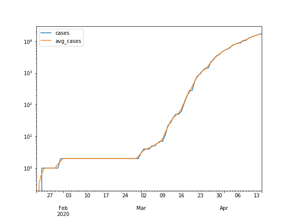
Finally we will create a couple of line plots. First, create one for DeKalb County that shows the number of cases versus the average number of cases. Next, create one for Cook County but use a log-scale for the y-axis. Note that you will be able to see the curve starting the flatten, showing that cases while still growing, are not doubling at the same rate.
Hints
- Make sure to use the correct frequencies for shifting and rolling. You must specify that you are shifting by days.
- To get the data for a specific county, you will need to use a
loccall that includes two levels of the index (e.g. both Illinois and DeKalb) - If you extract the cases and average cases at the same time, you can pass these to
plot.linedirectly so there is no need to set x or y arguments.
Extra Credit
- Draw a plot that compares Cook County to Los Angeles County
- Create a data frame that shows the new cases reported each week by county.
- Write code to use the latitude and longitude values in the JHU dataset to allow a user to find the counts of all cases within a specific region (e.g. the rectangle with an upper-left corner at (43.236334, -89.652084) and a lower-right corner at (41.258110, -86.746049)).